The idea behind the proximity table construction is to exploit the fact that the relative position of the sensors of a particle detector are fixed by construction. Thus, it is possible to pre-calculate a metric between the barycenters of the sensors that help during the graph construction.
Different metrics can be used and compared :
- Euclidian distance. Used in the traditional KNN algorithm, it is simply the euclidian distance between two hits
- Modified distance. The euclidian distance can be modified to cope with the geometry or the simmetry of the detector
- Correlation. Instead of using the distance, one can use the correlation of appearence of hits at different sensors.
The general algorithm to compute such a proximity table is summarized in the following pseudo-code:
Input :
  geometry (geom)
  optional simulations (simulations)

Output :
  proximity table (neighbors)

neighbors={}
for s1 in sensors(geom)
   neighbors{s1}={}
   for s2 in sensors(geom)
      d=criterion(s1,s2)
      neighbors[s1].append_sorted(s2,d)
return neighbors
Euclidian distance as a metric
The Euclidian distance is the traditionnal metric used to build the data graphs, for example in the K-nearest-neighbors (KNN) algorithm. K is a parameter of the algorithm designing the minimum connectivity of any node.
It can be computed easily from the cartesian coordinates of the sensors as stated in the following pseudo-code
def euclidian_distance(s1,s2)
  return sqrt((s1.x-s2.x)^2+(s1.y-s2.y)^2+(s1.z-s2.z)^2)
s1 and s2 are any two sensors from the detector and si.x, si.y and si.z are the Cartesian coordinates of the si sensor.
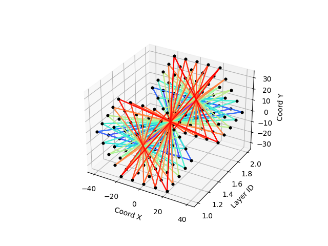
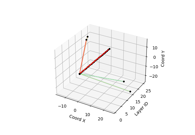
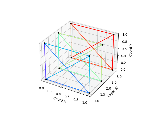
The following pictures show the result of the KNN algorithm on a one or two layers of calorimeter for K=2
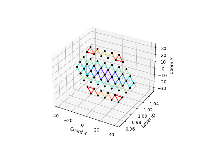
The typical problem of this metric is that it tends to create multiple non-connected components in the graph is K is low.
Distance modified by radiality : DIRAD-1
A modified distance can also be used, for example, a distance corrected by the radiality of the edge (the angle oriented by the longitudinal axis of the detector). The effect of such a metric is that it reduces the number of non-connected components as the graph is more oriented to the center of the detector, respecting its symmetry.
The following pseudo-code describes the concept
def dirad(s1,s2,alpha):
  d=euclidian_distance(s1,s2)
  mx=(s1.x+s2.x)/2
  my=(s1.y+s2.y)/2
  mz=(s1.z+s2.z)/2
  radiality=euclidian_distance((0,0,mz),(mx,my,mz))
  return d*(1+alpha*radiality)
Alpha is a parameter that adjust the radiality effect.
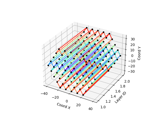
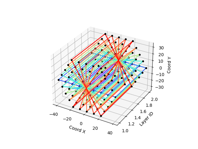
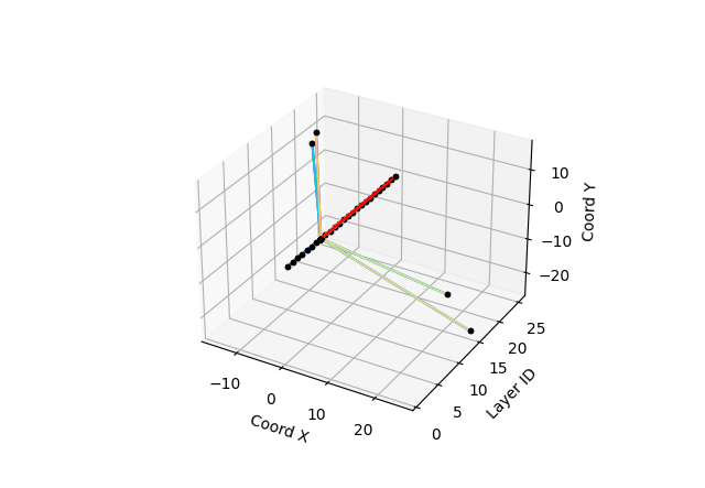
The following pictures show the result of the graph contructtion on a one or two layers of calorimeter for K=2 based on the DIRAD-1 distance
The effect of the alpha parameter is to inject more or less radiality in the construction. The next two figures show this effect for alpha=0.01 on the left (the result is similar to Euclidian) and alpha=0.4 on the right (full effect of radiality)
The drawback of this metrics is that the inter-layer connectivity is perturbed by the radiality.
Distance modified by radiality and layering : DIRAD-2
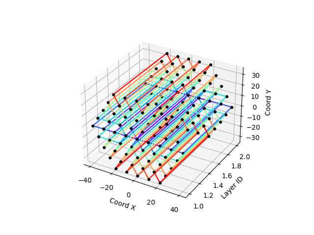
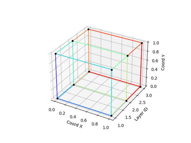
Instead of using modified distance for inter-layer and intra-layer construction, we can use a mix of them. Dirad-2 is using radiality corrected distance for intra-layer connectivity and Euclidian distance for inter-layer connectivity, clarifying the inter-layer connectivity as show in the new two pictures (DIRAD-1 on the left, DIRAD-2 on the right)
DIRAD-2 is a very good metric to used for layered detector with axial symmetry.
Correlation as a metric
Instead of using a distance as a metric, correlation can be used. Indeed, physical effects can induce distant but strongly linked measurements. In that case, it is legitimate to consider far events as strongly connected.
To calculate the correlation, a big bunch of events are analysed and the correlated measurements are counted in a table. This counting can be based on a simple counting (increment=1) or based on the energy deposition (increment=energy(si)). In the latter, the table is not symmetric. At the end of the counting process, a softmax is used to normalized the correlation in the 0:1 range.
The following pseudo-code implement such a correlation calculation
correlation=zeros(geom_size,geom_size)
for e in simulations :
for s1 in sensor_list(geom)
for s2 in sensor_list(geom)
if hit(s1,e) and hit(s2,e)
correlation[s1][s2]+=increment
correlation[s2][s1]+=increment
return softmax(correlation)
#corresponding distance
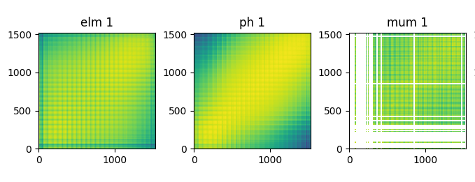
def corr_distance(s1,s2)
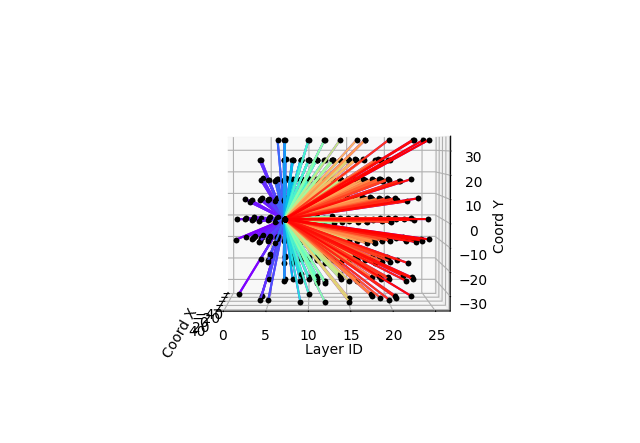
return correlation[s1][s2]The following figure show the correlation table in an electronic calorimeter for different kind of particles (electron, photon and muon)
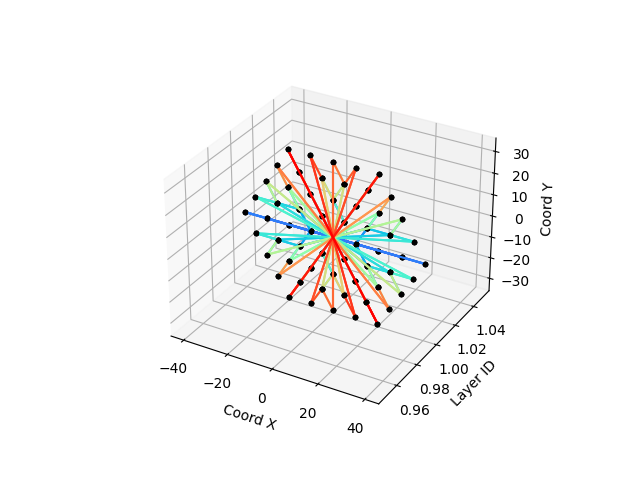
The corresponding graph construction gives very different graph from distance construction. Typically, the graph is oriented to the initial particle. The following figures show typical graph for an electron (on the left) and for a muon(on the right) for increment=1
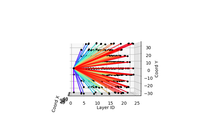
The following figures show typical graph for an electron (on the left) and for a muon(on the right) for the energy increment. This technique is more accurate in the sense that is focalize the graph on the main interactions of the event.
Proximity table cuts
The storage of the proximity table can be problematic if the detector is big because its size is the square of the number of sensors. It is possible to reduce its size by simply cutting it.
Different possibility are available to reduce the size of the table
- Cut by layers (isolate the noise)
- Cut by number of neightbors (best solution)
- Cut by distance (good rendition of detector physics but unpractical because the table size is not fixed)
The following figures show the impact of a layer cut on the graph construction (no cut on the left, layer cut on the right)
The advantage of this technique is to reduce dastically the mean complexity of the graph generation but also the size of storage of the proximity table. The main disadvantage is that it use increases the risk of non-connected components.