This dataset is a simplified simulation of a sampling calorimeter. It is inspired by the HGCal detector, the future endcap simulator for the CMS detector at LHC/CERN. CMS is a general detector (one of the four detectors of the LHC). It is composed of different layers gathering information about the events (proton-proton collisions). The calorimeter part evaluate the energy of the particles. It is composed of two parts. The barrel (the cylindrical part of the detector) and the two encaps.
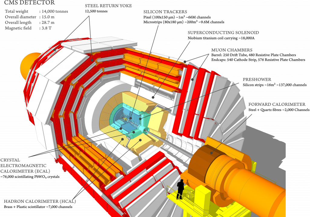
HGCal is the future replacement of the encap calorimeters. As a sampling calorimeter, it is composed of alternate layers of detectors (silicon or scintillator) and absorbers (metallic blocks). The particle are converted in the absorbers in shower of secondary particles. The sensor is made of pixels which give tracks of these showers. It is composed of two parts, an electromagnetic calorimeter (ECAL) for low mass particles (leptons) and a hadronic part (HCAL) for heavy particles (hadrons).
The shape of the showers give hints on the nature of the particule and its energy.
In the simulations, two kind of detectors are implemented (a third is in preparation)
d1 architecture
The d1 version of detector is a sampling electromagnetic calorimeter consisting of 25 pairs absorber-sensor placed at a 3 mm distance one from other along the Oz axis. The total length of the calorimeter is 22 cm and the diameter 90.0 mm. The sensor layers represent a silicon segmented into hexagon cells map. Each cell has a surface of about 1cm2 and thickness of 320 micrometers. The absorber plate is made of Pb and has a thickness of 5.6 mm. The following table summarize these informations.
| Nb layers | 25 |
| Nb rings | 5 |
| Layer spacing | 3.00 mm |
| Cell material | Si |
| Cell thickness | 0.32 mm |
| Cell diameter | 10.0 mm |
| Absorber plate material | Pb |
| Absorber plate thickness | 5.6 mm |
| Total length | 220.0 mm |
| Diameter | 90.0 mm |
d2 architecture
the d2 architecture is composed of electromagnetic and hadronic parts. This detector, designed for an optimal detection of electrons and photons of 100 GeV and hadrons of 200 GeV, consists of alternating pairs of absorber and silicon layers. The 26 Ecal absorber layers are made of lead and has a thickness of 6.05 mm, while the Hcal section has 24 absorber layers made of stainless steel, the first 12 with thickness of 45mm and the second 12 with a thickness 80.0 mm. All active silicon layers are transversely segmented into hexagon cells of 320 micrometers of thickness with surface of about 1 cm2 for the Ecal and 4 cm2 for the Hcal. The total transverse section of the Ecal has a diameter of 69 cm, while the Hcal has a diameter of 98 cm. These dimensions were chosen to insure at least 95% containment of the radial extension of the electromagnetic and hadronic showers. The pair of absorber and active layers are placed at a distance of 3 mm each from other, the total length of the calorimeter is 1.84 m with 0.24 m for the Ecal and 1.60 m for the HCal.
| ECAL | NEAR HCAL | FAR HCAL | TOTAL | |
|---|---|---|---|---|
| Nb layers | 26 | 12 | 12 | 50 |
| Nb rings | 35 | 25 | 25 | |
| Layer spacing | 3.00 mm | 3.00 mm | 3.00 mm | |
| Cell material | Si | Si | Si | |
| Cell thickness | 0.32 mm | 0.32 mm | 0.32 mm | |
| Cell diameter | 10.0 mm | 20.0 mm | 20.0 mm | |
| Absorber plate material | Pb | Stainless steel | Stainless steel | |
| Absorber plate thickness | 6.05 | 45.0 mm | 80.0 mm | |
| Length | 240.62 mm | 1576.68 mm | 820.46 mm | 1820.3 mm |
| Radius | 345.0 mm | 490.0 mm | 490.0 mm | 490.0 mm |
The simulations
We performed Geant4 simulation (geant4 10.5.1) to produce a set of data collected in a sampling calorimeter hit by different type of particles (electrons, photons, muons and pions). The calorimeter is placed along the axe Oz in an experimental chamber containing air. Monoenergetic single particle beam hits the detector with 0° incidence at (0,0,0).
The recorded data contain information about the incident particles, deposit energy and cell identification.
The data
The data are available at the address https://llraidata.in2p3.fr/hgcnn/
The simulations of each geometry are available in a dedicated folder (d1 or d2). Each folder contains similar files:
- geometry_d[i].dat : text file containing the coordinates of the barycenter of the sensors. The available fields are layer number, sensor identifier, x coordinate, y coordinate, z coordinate. This is the base file for the proximity table construction.
- The data of the events are stored in dedicated subfolders like elm_E50_theta0. The first part indicates the nature of the particle (elm for electron, mum for muon, pip for positive pions and ph for photons), the second part indicates the energy of the particles (in this case 50), it can be a single number or a range like 50-100, the last part indicates the incidence angle with respect to the longitudinal axis Oz.
- The primary particle parameters are available in the primaryParticle_d[i]_…_number.dat files. The “…” part is a copy of the folder name. The number indicates the index of the file. Indeed, to simplify the treatment, the simulations are grouped in files of 10000 events. Each line correspond to the primary particle associated to an event. The available fields of each line are event identifier, particle name, energy in GeV, two angles of incidence, the three coordinates of the first interaction between the particle and the detector and finally a global time. All these values can be used as labels for classification or regression
- The event data are in the file sensors_d[i]_…_number.dat. Each file consists in a collection of lines, each describing a hit. Note that a single event is composed of many hits. Thus a single event is represented by multiple lines beginning with the same event id. For each line, the fields are the event identifier, the sensor identifier, the energy deposited in the sensor and the three coordinates of the barycenter of the sensor. These data are typically the input for the neural network.
The loader
A loader is implemented in the reference code.