The graph readout is a function that map a graph with features in a fixed size vector. There are different way to implement this kind of function. It can be based on a simple association with random placement and zero-padding.

Here is an example of a simple flatten

def simple_flatten(graph g):
    i=0
    result=[]
    for each node n in g: #random ordering
        for each f in n.features
            result[i]=f
            i=i+1
     while i<output_size:
        result[i]=0
        i=i+1
     return result

This kind of implementation has two major drawbacks. First of all, the number of nodes of the graph has to be less than the output size. Thus, it leads to choose big vectors which will slow down the training of the MLP. Secondly, the random choice will lead to blurred inputs which prevent to get anything else than density detection or unordered pattern recognition.

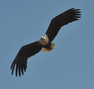
The following picture illustrate this difficulty, on the left, a bird picture, on the right the same image with its pixels shuffled. Obviously, even if all the information is present in the right image, it is impossible to recognize a bird. This is why it is very important to recreate an order at the readout time.

A first improvement can be achived by ordering the nodes in the “for each” instruction. It can be done for example on a hidden feature which is the identifier of the sensor. Nevertheless, the problem of the size of the output remains.

To prevent it, we can include a last pooling in the readout operation, by grouping some node that belong to the same place. Again this can be done, based on hidden feature. A good example is to store the x,y,z coordinates in the hidden features. During the readout operation, the detector is divided into geometric parts and all the nodes belonging to the same part will be fusion by a pooling operation.

def geometric_pooling_flatten(graph g, geometry geom):
    parts=partitioning(geom)
    result=[len(parts)*nb_features]
    for each node n in g: 
        p=belongsto(parts,n)
        p.pool(n) #fusion the features of n to other nodes of p 
    for p in parts:
        for f in features(p)
            result[i]=f
            i=i+1
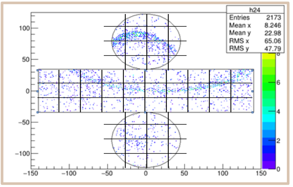
    return result

In this code, “partitioning” creates a partitionning of the sensor space. “belongsto” determine to which part a node belongs to. “p.pool” merge the node with the previous nodes with a pooling function. The next figure illustrate the partitionning of the Hyper-Kamiokande detector

This way, the size of the output vector is completely defined by the partitioning and the features vector lenght and can as small as we want. Inside this output vector, the values are ordered by the geometry itself.

Note that the disadvantage of this method is to break the symmetry of the detector. The effect of this symmetry breaking is that a lot more data is needed to train the network because, instead of learning a shape of object, it has to learn it at every position.

To correct this effect, a variant can be used. Instead of using absolute coordinates, we can use symmetry invariant values (for example, a high z and an angle refered to an event based reference for axial symmetry detector).