This algorithms takes an event as input and generates the corresponding graph based on the metric calculated in the proximity table.
Input :
  event (event)
  proximity table (neighbors)
  number of edge per node (K)

Output :
  event graph (result)

result=empty_graph()
for h1 in hit_list(event)
   result.add_node(h1)
for h1 in hit_list(event)
   for h2 in neighbors(h1)
      if nb_edges(h1)>K
          break
      if h2 in hit_list(event)
          result.add_edge(h1,h2)
return result
The add_node function creates a new node in the graph. This node get features from the event. These features must be choosen very carefully in order to bring enough information to the convolution operations but avoiding to include misleading informations. For example, it is often a good idea to remove the geometric coordinates to cope with the symmetry of the detector. These informations can be forgotten or stored in special memory that we called hidden features. These features will be stored but not modified by the convolution operation.
Thus a node should have a structure looking like
class node:
    neighbors[]
    edges[]
    features[]
    hidden_features[]
The add_edge function creates an edge in the graph. It takes two nodes as argument. Every edge has features. Again, the information provided should not break the symmetry. For example, the edge length (Euclidian distance between the sensors) is a good information. Hidden features can also be added (for example the cartesian coordinates).
An edge should have a structure like
class edge:
    node o,e #origin and end nodes
    features[]
    hidden_features[]
The following picture shows the graph generated from an electron event with the Euclidian distance
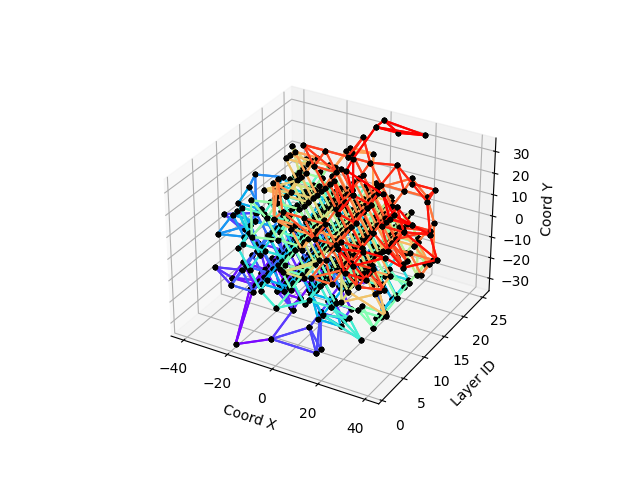
The complexity of the graph generation algorithm with Proximity tables is \mathcal{O}\left(\log^2(N)\right). A full proof can be found here.